
“I know that I know nothing”
– Socrates, according to Plato –
“I think, therefore I am”
– René Descartes –
I. Plato’s Allgory of the Cave
In the last weeks the allegory of the cave came often to my mind while investigating most recent approaches to better understand the learning mechanism within Deep Neural Networks (DNNs). This allegory by the Greek philosopher Plato is contained as a part in his work Republic (514a-520a) and compares “the effect of education and the lack of it on our nature”. The allegory is written in the form of a dialogue between Plato’s brother Glaucon and his mentor Socrates. In it, Socrates is the actual narrator and he first decribes the scenery to us as follows (source 1, source 2):
I.1. A Visual Picture by Socrates
“Behold! human beings living in an underground cave, which has a mouth open towards the light and reaching all along the cave; here they have been from their childhood, and have their legs and necks chained so that they cannot move, and can only see before them, being prevented by the chains from turning round their heads. Above and behind them a fire is blazing at a distance, and between the fire and the prisoners there is a raised way; and you will see, if you look, a low wall built along the way […] And do you see […] men passing along the wall carrying all sorts of vessels, and statues and figures of animals made of wood and stone and various materials, which appear over the wall? Some of them are talking, others silent. […] “
I.2. Act of Breaking Free
Socrates further clarifies how the cave prisoners might assert true existence to their sensual experiences:
“From the beginning people like this have never managed […] to see anything besides the shadows that are projected on the wall opposite them by the glow of the fire. […] And now what if this prison also had an echo reverberating off the wall in front of them? Whenever one of the people walking behind those in chains would make a sound, do you think the prisoners would imagine that the speaker were anyone other than the shadow passing in front of them? […] To them […] the truth would be literally nothing but the shadows of the images”

II. How Do Humans Gain Knowledge?
The image described in this analogy plays a key role in the history of philosophy and science. It touches the perhaps most fundamental question how we gain knowledge and understanding about the “true” causes of the observed phenomena through our senses. According to Plato, the philosopher is the prisoner who has managed to free himself from the imprisonment inside the allegoric cave. He or she has gained knowledge about the “true” causes of the projection shadows.
II.1. Human Senses – Uncertain Observations
As humans we observe the world through our natural senses and our brain then builds the knowledge and understanding upon these observations. Through centuries of human endeavor to gain knowledge about the world surrounding and containing us, we developed a plethora of tools and methods to broaden our natural senses. These extensions like measuring tools and mathematics just help us to extract knowledge from our sensual experiences in more systematical manner.
II.2. Systematic Knowledge Generation – Reducing Uncertainty
This is our never ending attempt to free ourselves from the virtual cave of ignorance. Forming intuitions about the causes of sensory phenomena, compress them into self-consistent theories, then actively test assertions of these theories on future sensory input and adapt the theories. In other words, our brain as our inference engine is bound to its own virtual cave and can only see, hear, taste and touch the outside world as shadows of the “true” causes projected to the walls of its prison. Consequently, all theories and models that we build based on our observations are constructed under uncertainty.
II.3. An Helpfull Perspective
This perspective will help us understand the process at play within Deep Learning (DL) in Artificial Neuronal Networks (ANNs). We then will see that DL is nothing else than just a very successful automated process by which information is extracted from a huge amount of diverse data and then successively compressed into more and more abstract and higher-order features that give shorter representations of the information contained in the input data set.
III. Information Theory – A Powerful Approach to Quantify Levels of Knowledge under Uncertainty
Taking on that perspective allows us to utilize a very powerful theory for quantifying information processing under uncertainty in a mathematically rigorous and quantifiable way. Information theory, originally proposed and developed by Claude Shannon in 1948, studies the quantification, storage, and communication of information. The impact of this theory, which is at the intersection of such different research fields like mathematics, statistics, computer science, physics, neurobiology, and many more, can not be underestimated. The key measure within information theory is the information entropy, also often called just entropy. The entropy measure quantifies the amount of uncertainty involved in a specific random process. It can also be interpreted as the average level of “information”, “surprise”, or “uncertainty” that is inherent in the (random) variable’s possible outcomes.
III.1. Entropy as a Measure of Uncertainty
In the context of the cave allegory and the situation of the prisoners, the act of breaking free from the cave is an attempt to maximally minimizing this information entropy by acquiring the “true” causes of the observed phenomena. Furthermore, when we humans try to build models upon our sensory observations, that is equivalently an approach to continuously minimize the amount of “uncertainty” (entropy) about the future.
III.2. Physical Theories as Compressed Knowledge
This brings us to another intriguing interpretation of information entropy, namely as information content. Particularly, a theoretical description or model which explains many phenomena in nature possesses high information content. As an example one can consider the four Maxwell equations of Electrodynamics. With these four equations alone it is possible to derive and thereby explain a fair deal of electromagnetic phenomena. Hence, we can say that the Maxwell equations possess high information content. There is actually a wired article on these amazing equations that nicley tries to explain their power and why physicists tend to be particularly in love with them.
III.3. More Information in a Shorter Message
When we talk about different levels of information content, we may consider also the notion of information compression. It leads us to ask how much information one is able to compress within a shorter optimal description of manifold observations, later allowing the reproduction of the original information. In the original purpose of the Information Theory, as developed by Shannon, a compression is said to be lossless, if the compressed message has the same information quantity as the original message, but carries this same amount of information in a much shorter message length.
IV. Information Theory of Deep Learning – Introduction
Information theory also builds the basis of a promising recent theoretical approach on describing the process of Deep Learning. This is called the Information Bottleneck (IB) theory and was mainly proposed and developed by Naftali Tishby and colleagues from the Hebrew University at Jerusalem. In summary, the IB theory describes the Deep Learning process as a procedure to compress a huge amount of data with all its features into a shorter representation. A neural network with all its neurons and intrinsic connection weights is in essence that short representation. Propagating any input from the same domain of the training data forward through the network at a later time then allows at best to extract the output information what this specific data sample represents.
IV.1. A Visual Example
For a visual explanation of the IB theory let us consider a network that was trained to represent a huge image data set containing cats and dogs. Later feeding another image containing either a cat or a dog as input to the DNN shall give as output the decision if there is a cat or a dog in the image. Tishby and Zaslavsky formulate in their 2015 paper “the goal of deep learning as an information theoretic tradeoff between compression and prediction”. They further state that “the goal of any supervised learning is to capture and efficiently represent the relevant information in the input variable about the output – label – variable. Namely, to extract an approximate minimal sufficient statistics of the input with respect to the output”. Or to put it differently: “find a maximally compressed mapping of the input variable that preserves as much as possible the information on the output variable”.
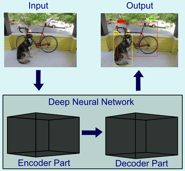
IV.2. Deep Neural Networks – Encoders and Decoders of Information
Here, in accordance with Tishby and colleagues, the consideration of a DNN as two-part system is made (see Figure 1). The first part, the Encoder, extracts relevant information from the input data set. The second part, the decoder, decodes the output class (human, animal, other objects) from the extracted features represented within the encoder. The sample input and output images in Figure 1 represent the so-called YOLO v3 algorithm. This specific (convolutional) DNN was trained on images to extract distinct object classes together with the corresponding bounding boxes around the objects in the image. The abbreviation stands for “You only look once”, specifying that the algorithm is able to process the image once and extract all objects in parallel in one pass through the DNN.
V. Information Theory of Deep Learning – Basic Definitions and Main Properties
Typically, the input is high-dimensional. For example consider a large and diverse image data set with samples containing people, animals, nature, buildings, etc. Principally, there is a considerate amount of information contained in such an image, and even more information is consequently contained in a data set of thousands to millions of images. However, in line with the central goal of deep learning, we are just interested in detecting the object classes in this information diverse data. If a functional mapping from the high-dimensional input to the singular object detection and classification (low-dimensional decision of class number $0,1,2,\ldots,N$ , with being a natural number) exists, then it yields the intuition that most of the information entropy within the input must be “irrelevant” to the decision. Thus, the ultimate goal of deep learning will be to extract those “relevant” features (information) out of the sea of irrelevance.
V.1. Kullback-Leibler Divergence – A Measure of Distance Between Probability Distributions
The information, that an input random variable $X$ (image) contains about an output random variable $Y$ (specific object in image), is mathematically represented by the mutual information measure, $I\left( X;Y \right)$. Before we define mutual information, we have to first introduce the relative entropy or Kullback-Leibler Divergence as a measure of distance between two probability distribution functions $p\left( x \right)$ and $q\left( x \right)$, which is defined as
\begin{equation} \label{eq:kullback_leibler}
D\left(p||q\right)=\sum_{x\in X}p\left(x\right)\log\left(\frac{p\left(x\right)}{q\left(x\right)}\right).
\end{equation}
V.2. Mutual Information – Or What Can Be Known About One Random Variable From Another Random Variable
It can be shown that the relative entropy is always non-negative and is zero if and only if the involved probability distributions are equal ($p = q$) [Cover and Thomas (2006)]. Now, we can define mutual information: Let $X$ and $Y$ be two random variables with a joint probability distribution function $p\left( x, y \right)$ and the corresponding marginal probability distributions $p\left( x \right)$ and $p\left( y \right)$. The mutual information $I\left( X;Y \right)$ is the relative entropy between the joint distribution and the product distribution $p\left( x \right) p\left( y \right)$:
\begin{align}
I\left(X;Y\right) & =D\left[p\left(x,y\right)||p\left(x\right)p\left(y\right)\right]\\
& =\sum_{x\in X}\sum_{y\in Y}p\left(x,y\right)\log\left(\frac{p\left(x,y\right)}{p\left(x\right)p\left(y\right)}\right).
\end{align}
With the definition of relative entropy at our disposal, we readily see that the mutual information between $X$ and $Y$ is always positive and just zero, if and only if $p\left( x,y \right) = p\left( x \right) p\left( y \right)$ for all $x \in X$ and all $y \in Y$. As a consequence, the random variables $X$ and $Y$ would be conditionally independent in this case. Coming back to our problem of representation learning within DNNs, $X$ is our input space and $Y$ our output space. Hence, the mutual information necessarily should be nonzero, otherwise the whole approach to find a minimal sufficient mapping (statistics) from input (image) to output (class affiliation) would fail.
V.3. First Important Property Of Mutual Information – Transformations that Preseve Information
Definition
From the definition of the mutual information two properties follow which are important in the context of DNNs. First, the information captured by the network is invariant under invertible transformations:
\begin{equation}
I\left(X;Y\right)=I\left(\psi\left(X\right);\phi\left(Y\right)\right)
\end{equation} for any invertible functions $\psi$ and $\phi$. Mathematically, this means that for two elements $x$ and $x’$ in $X$, we have $x’= \psi \left( x \right)$. Then, the inverse function $\psi ^{-1}$ exists, such that $x = \psi ^{-1} \left( x’ \right)$.
A Visual Example
Examples of (linear) invertible transformations are spatial translations and rotations. Consider for visualization purposes that we take one sample image (e.g. the image in Figure 1) and rotate it $90°$ clockwise ($\psi$). Then the inverse operation is the application of $90°$ rotation anti-clockwise ($\psi ^{-1}$). This example explains the empirical observation that some DNNs fail to correctly classify objects in images if the image is rotated. That can be circumvented by including several transformed versions of the same data samples in the training data set. Otherwise, the transformed samples will be outside of the input space $X$ ($x’=\psi\left(x\right)\notin X)$) and the corresponding information can not be represented within the DNN.
V.4. Second Important Property Of Mutual Information – Data Processing Inequality
Markov Chains
The second important property is the Data Processing Inequality (DPI). To define the DPI, we have to first introduce the notion of a Markov chain [Cover and Thomas (2006)]: Random variables $X$, $Y$, $Z$ form a Markov chain $X\rightarrow Y\rightarrow Z$ if the conditional distribution of $Z$ depends only on $Y$ and is conditionally independent of $X$. Equivalently the joint probability distribution function of all three variables can be written as
\begin{equation}
p\left(x,y,z\right)=p\left(x\right)p\left(y|x\right)p\left(z|y\right),
\end{equation} for all $x\in X$, $y\in Y$ and $z\in Z$. Translating this concept to our DNN, the layers, $T_{1},T_{2},\ldots,T_{M}$ ($M$ being the number of layers) of the DNN then form a Markov chain:
\[T_{1}\rightarrow T_{2}\rightarrow T_{3}\rightarrow\cdots\rightarrow T_{M-1}\rightarrow T_{M}.\] This is exactly how Tishby and colleagues formulated the DNN within the IB theory.
Definition of Data Processing Inequality
With the introduction of the Markov chain, we can now formulate the DPI: If $X\rightarrow Y\rightarrow Z$ for three random variables $X$, $Y$, $Z$, then it holds $I\left(X;Y\right)\geq I\left(X;Z\right)$. Again, transforming this concept to the case of the DNN yields the following DPI chain: \begin{equation}
I\left(X;Y\right)\geq I\left(T_{1};Y\right)\geq I\left(T_{2};Y\right)\geq\ldots\geq I\left(T_{M};Y\right)\geq I\left(\hat{Y};Y\right).\label{eq:DPI_DNN} \end{equation} Here, $Y$ denotes the true (ground-truth) class label, while $\hat{Y}$ is the predicted class label by the network.
A Visual Understanding of Data Processing Inequality
Yet, this chain of information processing can be read and understood as follows: The initial mutual information content between the input $X$ and the true labels $Y$ is the highest, containing the whole sea of features (relevant and irrelevant). From layer to layer the information is compressed continuously. The first layer captures for example information at the pixel level (like edges, colors, etc.), the second layer combines these lower-level features to more abstract features (e.g. body parts, object parts, etc.), thus it holds less information content than the previous layer. Equivalently, the process approaches to the lowest information content at the last layer.
VI. Information Theory of Deep Learning – The Information Plane
To better understand the IB theory in general and how the concept of mutual information captures the essence of deep learning, Tishby and co-workers utilized the concept of information plane. Graphically, the information plane is visualized as a two-dimensional Carthesian plane (see Figure 2).
VI.1. Information Plane – Introduction
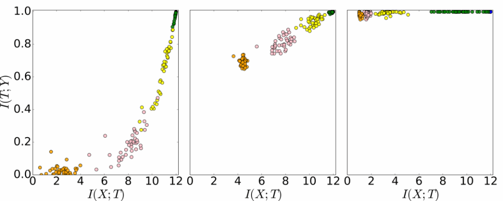
In the information plane, the $x$-coordinate axis is taken by the mutual information, $I_{X}=I\left(X;T\right)$, between the input $X$ and the neural network representation $T$. Simply put, it is just a quantitative measure for the amount of information about the input stored in the network layers with all the neurons and the connection weights between any two neurons. The $y$-coordinate axis then represents the information about the output $Y$ stored in the network representation $T$, being the mutual information measure $I_{Y}=I\left(T;Y\right)$. Most importantly, the mutual informations $I_{X}$ and $I_{Y}$ serve as order parameters governing the dynamics of DNNs during the learning process. To understand this dynamics, it is then only needed to hold track of these two mutual information measures while dismissing the dynamics of any layer or even any neuron itself.
VI.2. A Powerful Tool to Visualize Training of Network Ensembles
The information plane allows us to visualize the complete training life cycle of tens to hundreds of neural networks with potentially different architectures and different initial weights. Specifically, we can see that in Figure 2, where the process of the training is visualized for $50$ randomized neural networks during the whole training process on the same data set. Here, the differently colored circles represent different layers, with the green circles being the first layers after the input, yellow the second layers, up until orange being the last layers just before the output. As we observe, the first layers contain the most information both about the input and the output at the beginning of the training process, in accordance to the DPI chain above. In contrast, the last layer has nearly zero information about both the input and the output.
VII. Information Theory of Deep Learning – Two Phases of Learning
VII.1. Fitting Phase – Putting Labels to Data
Yet, a very interesting phenomenon emerges for all the randomized networks, independent of initialization. Within the smallest fraction of the overall training life-cycle the network starts to capture more and more information about both the input and the output in all layers. This is observed by the circles of the deeper layers going from the lower left corner to the upper center of the information plane. Tishby and colleagues characterized this phase of the training cycle as the fitting phase. Within that phase, each input is just fitted to the corresponding output labels. After a phase transition into a second phase (compression phase), the deeper layers continuously capture more and more information about the output through training. That is observable by the corresponding circles going up in $I_{y}$-direction, while the motion in $I_{x}$-direction is pointing more and more in direction to lower information about the input.
VII.2. Compression Phase – Forgetting Irrelevant Information
Generally, after many learning epochs information about the input within all layers is gradually decreasing. One can imagine this process as a kind of forgetting procedure. Let us consider the example of human detection in images. In the fitting phase, the network might just consider any type of image feature as relevant for the classification. For example it may be that the first batches of the training data set contain mostly images of people at streets in cities. Hence, the network probably will memorize such features as important for the task of detecting humans in the image. Later it might see other samples with people inside houses, people in the nature and so on. It shall then “forget” these too specific features. We can somehow say that the network have learned to abstract away the specific surrounding environment features to an extent that it generalizes well over several image samples.
VIII. Information Theory of Deep Learning – Analogy to Statistical Theory of Thermodynamics
VIII.1. Macroscopic versus Microscopic Description
From an empirical perspective, the ability of deep artificial neuronal networks to generalize well is very much known. However it is mostly only the case as long as we supply sufficiently large and diverse amounts of training data, put a lot of effort in designing and iteratively tuning network architectures and a lot more. But, it is thanks to the IB theory that enables a way more rigorous study of deep learning generalization. The consideration of the mutual information and the concept of the information plane shows clearly that the deep learning process within DNNs can be well described with the aid of “macroscopic” order parameters like the mutual information instead of the “microscopic” parameters like specific connection weights at one specific neuron at a specific hidden layer (out of maybe more than hundred layers).
VIII.2. Analogy with Statistical Thermodynamics
Certainly, DNNs possess parameters (neural connection weights and biases) up to billions in number. Yet, the IB theory delivers a description picture with two parameters (the two axes of the information plane) instead. This picture is reminiscent of the statistical theory of thermodynamics in physics. Typically, one can characterize a thermodynamic system by the dimensionless Avogadro number, $N_{A}\approx6.02\times10^{23}$, which is the number of particles (e.g. molecules, atoms or ions) within one mole of a material (a number with $23$ zeros). Describing the dynamics of such a system by taking into account the dynamics of all particles at each moment in time is simply not feasible. Hence, the thermodynamic theory considers macroscopic state parameters like temperature, pressure and volume for a more effective description. As a consequence, a specific set of values for these thermodynamic state variables can correspond to infinite configurations of the microscopic.
VIII.3. A Visual Example – Putting Milk into Coffee
Let us discuss the visual thought experiment with a cup of coffee. For a specific temperature of the hot beverage, the constituent particles are moving randomly around. When we measure the locations and momenta for each particle at a specific time, then we have the microscopic configuration related to this time moment and temperature. Measuring the microscopic states (locations and momenta) for each of the particles again at a later time gives us another microscopic configuration related to the same macroscopic variable value (temperature). But let us just assume the single particles to be interchangeable. Thus, in thought, we shall exchange particle locations and momenta with each other such that the previous configuration is yielded. From that perspective, there is no sense in considering the constituent particle’s states and we can just stick to the macroscopic description.
VIII.4. Ensemble of Networks Trained on the Same Data – What Do They Have in Common?
There is now an equivalent description level at play within the IB theory for Deep Neural Networks. In essence, Tishby and colleagues have shown that the several randomized networks pass through the same two training phases, over a phase transition from fitting to the compression phase. All the single networks that were trained for the experiment shown in Figure 2 pass through similar information plane regions along similar information dynamical trajectories, though each of them have completely distinct random initialization of the connection weight parameters. Moreover, the architecture of each of these randomized networks can differ, the numerical values of specific connection weights may also differ, and the location of one neuron that encodes a specific feature (e.g. particular type of edges or colors) can be at one place in a layer for one network and in another location for the other network.
VIII.5. Describing All Network Weights = Trying to Track All Molecules in a Coffe Pot
In final consequence of the analogy to thermodynamic systems, the macroscopic state represented by a point in the information plane possesses infinitely many configurations at the microscopic level of all neuron states at all hidden layers. In that sense, trying to understand a DNN by considering the individual states of each neuron is as if we want to understand and describe a cup of coffee by measuring the locations and momenta of each particle in the fluid at each moment in time, an endeavor principally possible but practically infeasible.
IX. Conclusion and Outlook
In this first part, the Information Bottleneck (IB) theory as an approach to understand Learning in modern Deep Neuronal Networks (DNNs) was discussed. We saw that at the core of IB is information theory. Moreover, we saw in what terms the theory delivers a better understanding with just two macroscopic parameters instead of microscopic level parameters of the DNNs. Lastly, it was argued that an analogy between these two mutual information measures to macroscopic variables in statistical thermodynamics exists.
In a next part more details of the IB theory will be provided. Firstly, I will examine the question what role the size of training data plays. We will then see to what extent the two phases of the stochastic gradient descent (SGD) optimization are akin to the drift and diffusion phases of the Fokker-Planck equation. This is another intriguing similarity to statistical mechanics.