
I. Introduction
I.1. A view back – what we have learnt
In the first part of this article, I introduced the Information Bottleneck (IB) theory as an approach to understand Learning in modern Deep Neuronal Networks (DNNs). We saw that at the core of IB is information theory. Moreover, we saw in what terms the theory delivers a better understanding with just two macroscopic parameters instead of microscopic level parameters of the DNNs. Lastly, an analogy between these two mutual information measures to macroscopic variables in statistical thermodynamics was discussed.
I.2. A view forward – what we will learn
Here, I provide more details of the IB theory. Firstly, I will examine the question what role the size of training data plays. We will then see to what extent the two phases of the stochastic gradient descent (SGD) optimization are akin to the drift and diffusion phases of the Fokker-Planck equation. This is another intriguing similarity to statistical mechanics.
II. The role of training data – how much is enough
One of the major results of the IB theory is the two phases of deep learning, a fitting and a compression phase. An intriguing observation was that the different randomized networks follow the same trajectories on the information plane, through the same two phases. As a consequence, Tishby and colleagues average over these trajectories of different networks and get an image like the one shown in Figure 1.

The figure illustrates training dynamics for randomized DNNs on 5%, 45% and 85% of the training data, respectively. Evidently, the fitting phase is equal in all the three cases. Opposed to that, inclusion of more data in training changes the compression phase characteristic.
Hence, small training sets lead to larger compression of layer information about the label $Y$. This is a sign of overfitting. Therefore, compression aids in simplifying the layer-wise representations, but it can also promote over-simplification. Note that the balance between simplification and not loosing too much relevant information is still a matter of investigation by Tishby and colleagues.
III. A Thought Experiment – An Excursion to Statistical Mechanics
Let us take a step back and talk about a completely different stuff. Or is it maybe not completely different? Let us do an experiment. We will do it in our head, a thought experiment, something theoretical physicists often make.
III.1. Drift and Diffusion – Or putting Color into Water
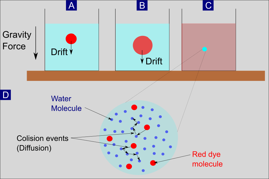
Our thought experiment goes as follows: We take a glass and fill it with water. Then, we dissolve a drop of red dye in the central upper part of the water (Figure 2 A). Due to the acting gravity force, the dye droplet drifts on average to the lower part in time.
At the same time, by a process called diffusion, the volume with dye molecules gets larger (Figure 2 B). As a final consequence of both processes, drift and diffusion, the dye molecules will be homogeneously distributed in the water. It has to be noted that there is already drift present without any external potential.
We will see later on, in case of the classical Langevin equation, that a drift occurs due to the friction force. The consideration of the gravity as external force is just for better illustration.
III.2. Individual Particle versus Ensemble of Particles – Two Sides of the same Coin
Yet, how shall we understand these two processes. Where might we even start with? Should we try to understand what the individual dye molecules do? Or shall we moreover ask how the dye droplet as a whole behaves in time? These questions lie at the core of statistical mechanics.
In statistical mechanics, we consider dynamics of systems that might consist of a huge amount of particles. One example was discussed in part one with the thought experiment on the coffee cup. Another example is the one illustrated in our current thought experiment.
Applying statistical mechanics on these systems shows in essence that both descriptions, microscopic versus macroscopic, are equivalent.
Contemplation on the problem date back even to roman times. In his first-century BC scientific poem, De rerum natura, the roman poet and philosopher Lucrecius described a phenomenon that we now know as Brownian motion.
Essentially, Lucrecius depicted the apparently random motions of dust particles as consequences of collisions with the surrounding air molecules.
He used this as a proof for existence of atoms. To be more precise, his illustration entails not solely the random part of the motion, but also the deterministic part of the dynamics. The latter part of the motion, caused by air currents, is comparable to the drift dynamics in our thought experiment.
The random part of the motion is attributed as Brownian motion, in honor of the scottish botanist Robert Brown. A simulation of the brownian motion is illustrated in Figure 3.

III.3. Single Particle Perspective – Stochastic Differential Equations
The single particle dynamics within Brownian motion is mathematically described through a stochastic differential equation (SDE).
Langevin Equation – Original Definition
A special instance of an SDE is the Langevin equation. This SDE was proposed by French physicist Paul Langevin. The original Langevin equation models the brownian dynamics of a particle in a fluid with a differntial equation for the particle velocity,
\begin{equation}
\frac{d\mathbf{v}}{dt}=-\gamma\mathbf{v}+\frac{1}{m}\mathbf{f}\left(t\right).
\end{equation} Here, we have the particle mass $m$ and its corresponding velocity vector in three spatial dimensions, $\mathbf{v}= \left( v_x , v_y , v_z\right) ^T$.
Langevin Equation – Two Terms
The Langevin equation possesses two terms, the first of which is the viscous (frictional) force proportional to particle’s velocity (Stoke’s law),
\begin{equation}
\mathbf{f}_{\text{fric}}=-m\gamma\mathbf{v}(t).
\end{equation} The factor $\gamma$ is determined by properties of the particle. The second term in the Langevin equation is a random force, $\mathbf{f}$. It models the consecutive collisions of the particle with the surrounding fluid particles and has a Normal distribution with its mean and two-time correlation being
\begin{eqnarray*}
\left\langle\mathbf{f}\left(t\right)\right\rangle & = & 0,\\
\left\langle \mathbf{f}\left(t\right)\mathbf{f}\left(t’\right)\right\rangle & = & \sigma\delta\left(\tau\right),
\end{eqnarray*} with $\tau = t – t’$. Hence, the correlation of the stochastic force is only non-zero, if the force at a time $t$ is completely uncorrelated with the force at any other time $t’$. More precisely, it is assumed that a correlation time $\tau_c$ exists, such that the stochastic force is non-zero for $\tau < \tau_c$.
Fluctuation-Dissipation-Theorem
The coefficient $\sigma$ is a measure for the strength of the mean square variance for the stochastic force. Since the friction also depends on the collisions, it should exist a connection between the noise intensity $\sigma$ and the friction coefficient $\gamma$. By solving the above Langevin equation, we can derive this connection, which is a special case of the Fluctuation-Dissipation-Theorem:
\begin{equation}
\sigma=2\gamma mk_{B}T
\end{equation} Here, $k_B$ is Boltzmann’s constant and $T$ is the temperature of the fluid. The assertion of the Fluctuation-Dissipation-Theorem is that the magnitude of the fluctuations (motion variance, $\propto \sigma$) is determined by the magnitude of the (energy) dissipation ($\propto \gamma$).
Langevin Equation in an External Potential
As a generalization of the original Langevin equation we can assume an external potential as addition. Henceforth, we arrive at the situation illustrated in Figure 2. There, we considered the existence of gravity pointing downwards. In classical Newtonian physics, gravity force is regarded as gradient of a gravity Potential. More generally, a potential force in one spatial dimension $x$ is defined as $F = -\partial _x U$. Herein, $U(x)$ is the potential function and $\partial _x$ is the partial derivative with respect to space coordinate $x$. With this, we yield the general Langevin equation in an external force field:
\begin{equation}
m\ddot{x}=-m\gamma\dot{x}-\frac{\partial U}{\partial x}+f\left(t\right),\end{equation} with $\dot{x}$ being the first time-derivative (velocity) and $\ddot{x}$ being the second time-derivative (acceleration). For simplicity, we restrict the investigation here to one spatial dimension $x$.
Overdamped Langevin Equation
A special case of the general Langevin equation in an external force field is the overdamped equation. We yield it by the assumption that the friction $\gamma$ shall be very high. As a consequence, it is $\gamma \dot{x}\gg \ddot{x}$. Hence, the overdamped Langevin equation is
\begin{equation}
\dot{x}=-\alpha\frac{\partial U}{\partial x}+\Gamma\left(t\right),\end{equation} with
\begin{eqnarray*}
\alpha=\frac{1}{m\gamma} & \text{and} & \Gamma\left(t\right)=\frac{1}{m\gamma}f\left(t\right).
\end{eqnarray*} The stochastic force $\Gamma\left(t\right)$ fulfills analogous relations for mean and correlation like the original Langevin equation stochastic force $f\left(t\right)$:
\begin{eqnarray*}
\left\langle\Gamma\left(t\right)\right\rangle & = & 0,\\
\left\langle \Gamma_{i}\left(t\right)\Gamma_{j}\left(t\right)\right\rangle & = & \sigma\delta\left(\tau\right),
\end{eqnarray*} with $\tau = t – t’$ and $\sigma = 2\alpha k_B T$.
General Stochastic Differential Equation (SDE)
Let $X\left(t\right)$ be a random variable, then we can define a general SDE as
\begin{equation}
\dot{X}\left(t\right)=h\left( X,t\right) + g\left( X,t\right) \Gamma \left(t\right),
\end{equation} with $h\left( X,t\right)$, $g\left( X,t\right)$ being some arbitrary, yet unknown functions, depending on $X$ and $t$. Furthermore, we have again a Gaussian white noise process $\Gamma\left(t\right)$ with the properties
\begin{eqnarray*}
\left\langle\Gamma\left(t\right)\right\rangle & = & 0,\\
\left\langle \Gamma_{i}\left(t\right)\Gamma_{j}\left(t\right)\right\rangle & = & 2\delta\left(t-t’\right).
\end{eqnarray*} The stochastic process $\Gamma\left(t\right)$ is called Wiener process in honor of the American mathematician Norbert Wiener for his investigations on the mathematical properties of the one-dimensional Brownian motion.
III.4. Ensemble Description – Fokker-Planck Equation
After scrutinizing the dynamics of single particles, we arrived to a description picture with SDEs. We can simulate thousands to millions of suspension particles moving within a glass containing another million to billions of smaller water molecules. The initial starting configuration might be the larger particles concentrated in a small area of the water (as in Figure 1). Henceforth, an individual SDE determines temporal dynamics for each suspension particle. In essence, that is what the Monte Carlo method is achieving as one major successful computational algorithm in statistical mechanics.
A Change of Perspective
But what if we just zoom out from the microscopic view up to a much more coarse-grained picture. From this high-ground view, the millions of particles will be smeared out to a distribution. Yet, the mathematical description also changes. Instead of millions of SDEs, we will have one deterministic partial differential equation to describe the macroscopic distribution of all particles in time and space. This macroscopic evolution equation is widely known as the Fokker-Planck equation. The crucial point is that, though the time evolution of each single particle is completely random, the particle population as a whole evolves deterministically.
Fokker-Planck Equation – Definition
For simplicity, we will limit the consideration to one spatial dimension $x$. Let $\rho\left( x, t\right)$ denote the particle distribution density at position $x$ and time $t$. Then, the Fokker-Planck evolution equation can be written as
\begin{equation}
\frac{\partial}{\partial t}\rho\left(x,t\right)=-\frac{\partial}{\partial x}\left\{ D^{(1)}\left(x,t\right)\rho\left(x,t\right)\right\} +\frac{\partial^{2}}{\partial x^{2}}\left\{ D^{(2)}\left(x,t\right)\rho\left(x,t\right)\right\}.
\end{equation} The equation possesses two coefficients that in general cases depend both on space and time. The first coefficient, $D^{(1)}\left(x,t\right)$, is called drift and the second, $D^{(2)}\left(x,t\right)$, is the diffusion coefficient. Note that the latter is always positive, $D^{(2)}\left(x,t\right)>0$.
Historical Context
The Fokker-Planck equation was first derived to describe Brownian motion from an ensemble perspective by the Dutch physicist and musician Adriaan Fokker and the famous German physicist Max Planck. Morover, it is also known under the name Kolmogorov forward equation, due to Russian mathematician Andrey Kolmogorov.
He devoloped the concept independently in 1931. Sometimes it is also called the Smoluchowski equation, after the Polish physicist Marian Smoluchowski, or the convection-diffusion equation. The latter is the case, when considering particle position distributions.
Derivation Outline
The Fokker-Planck equation can also be derived from a Langevin type SDE by building the Kramers-Moyal expansion of the distribution $\rho\left(x,t\right)$. Furthermore, the Kramers-Moyal Forward expansion scheme allows derivation of much more general evolution equations for any probability density $\rho\left(x,t\right)$, with infinitely many expansion terms on the right-hand side:
\begin{align}
\frac{\partial}{\partial t}\rho\left(x,t\right)= & \frac{\partial}{\partial x}\left\{ D^{(1)}\left(x,t\right)\rho\left(x,t\right)\right\} +\frac{\partial^{2}}{\partial x^{2}}\left\{ D^{(2)}\left(x,t\right)\rho\left(x,t\right)\right\} \\
& +\frac{\partial^{3}}{\partial x^{3}}\left\{ D^{(3)}\left(x,t\right)\rho\left(x,t\right)\right\} +\cdots+\frac{\partial^{n}}{\partial x^{n}}\left\{ D^{(n)}\left(x,t\right)\rho\left(x,t\right)\right\} \\
& +\cdots\\
= & \sum_{n=1}^{\infty}\left(\frac{\partial}{\partial x}\right)^{n}\left\{ D^{(n)}\left(x,t\right)\rho\left(x,t\right)\right\} .
\end{align} The Kramers-Moyal coeffcients $D^{(n)}\left(x,t\right)$ can be calculated with the given SDE for a random variable $X$ as follows:
\begin{equation}
D^{(n)}\left(x,t\right)=\frac{1}{n!}\lim_{\tau\rightarrow\infty}\frac{1}{\tau}\left\langle\left[X\left(t+\tau\right)-x\right]^{n}\right\rangle|_{X\left(t\right)=x}.
\end{equation} Herin, $X\left(t+\tau\right)$, with $\tau>0$, is a solution for a specific SDE which at time $t$ has the sharp value $X\left(t\right)=x$. Furthermore, for a variable $A$ the notation $\left\langle\left[A\right]^{n}\right\rangle$ denotes the nth moment of $A$. Particularly, the first moment is the mean and the second moment is the variance of $A$.
Derivation for General SDE
Let us consider the general SDE that we learned about previously, \begin{equation}
\dot{X}\left(t\right)=h\left( X,t\right) + g\left( X,t\right) \Gamma \left(t\right),
\end{equation} as an illustrative example here. We have assumed the Langevin type random force $\Gamma\left(t\right)$ to be a Gaussian (normal) distributed random variable. As such, it possesses zero mean and $\delta$-distributed correlation function,
\begin{eqnarray*}
\left\langle\Gamma\left(t\right)\right\rangle & = & 0,\\
\left\langle \Gamma_{i}\left(t\right)\Gamma_{j}\left(t\right)\right\rangle & = & 2\delta\left(t-t’\right).
\end{eqnarray*} Recognizing these properties yields the first and second Kramers-Moyal coefficients as the drift and diffusion coefficients of the Fokker-Planck equation, respectively. Notably, all other coefficients ($n\geq3$) vanish to zero. In summary, we have for the general SDE of Langevin type: \begin{eqnarray*}
D^{(1)}\left(x,t\right) & = & h\left(x,t\right)+\frac{\partial g\left(x,t\right)}{\partial x}g\left(x,t\right),\\
D^{(2)}\left(x,t\right) & = & g^{2}\left(x,t\right),\\
D^{(n)}\left(x,t\right) & = & 0\,\,\,\text{for all}\,n\geq3.
\end{eqnarray*}
Noise-induced Drift
An intriguing result here is that besides the determinsitic drift $h\left(x,t\right)$, the first coefficient $D^{(1)}\left(x,t\right)$ also contains an additional term. This added term stems from the random force part and consequently is called the noise-induced drift. This can be formulated in terms of the diffusion coefficient $D^{(2)}\left(x,t\right)$ as follows: \begin{equation}
D_{\text{noise}}^{(1)}=\frac{\partial g\left(x,t\right)}{\partial x}g\left(x,t\right)=\frac{1}{2}\frac{\partial}{\partial x}D^{(2)}\left(x,t\right).
\end{equation}
Fokker Planck Equation as a Continuity Equation
There is a visually appealing reformulation of the Fokker-Planck equation as a continuity equation:
\begin{equation}
\frac{\partial}{\partial t}\rho\left(x,t\right)=-\frac{\partial}{\partial x}j\left(x,t\right),
\end{equation} with \begin{equation}
j\left(x,t\right)=D^{(1)}\left(x,t\right)\rho\left(x,t\right)+\frac{\partial}{\partial x}\left\{ D^{(2)}\left(x,t\right)\rho\left(x,t\right)\right\}.
\end{equation} If we acknowledge $\rho\left(x,t\right)$ as a particle density or a probability density, then $j\left(x,t\right)$ plays the role of a particle flux or a probability flux, respectively. Continuity equations play a fundamental role all over theoretical physics. In essence, the statement of the continuity equation is that what goes out must be matched by what comes in. Best we can visualize this by a schematic picture shown in Figure 4.
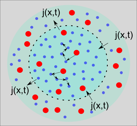
In here we again have the diffusion situation shown previously in Figure 2D. Now we see an inner circle that is separated from an outer circle by the dashed black boundary. If we consider the density of red dye particles inside the inner circle as $\rho\left(x,t\right)$, then a change in time for this density (left-hand side of the continuity equation) is generated through particle fluxes through the dashed boundary (right-hand side of the continuity equation).
IV. Back to IB Theory – Constructing the Analogy
So, after our tour-de-force through statistical mechanics of drift and diffusion processes the question is how this might help us in understanding Deep Learning.
IV.1. The Drift and Diffusion Phases of SGD optimization
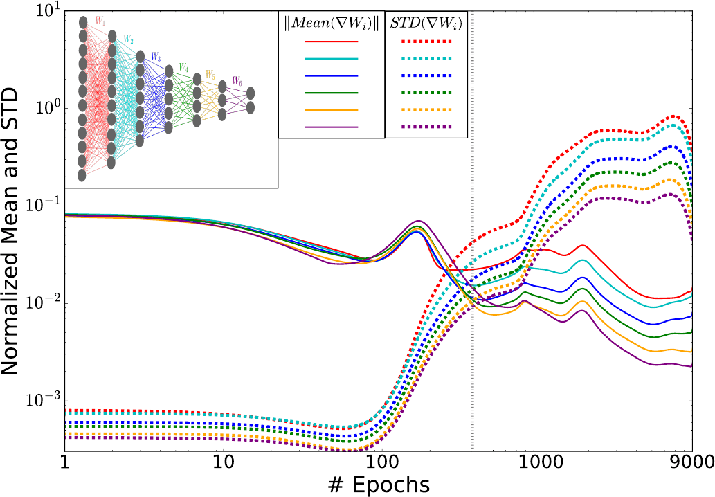
Training of neural networks often is achieved on small batches of training data by utilizing stochastic gradient descent (SGD) optimization. Tishby and colleagues have presented in their 2017 work a nice visual picture on the existence of such drift and diffusion phases during the SGD optimization.
For that, they calculated the mean and standard deviations of the weights’ stochastic gradients for each layer of the DNN and subsequently plotted these as functions of the training epoch (Figure 5).
IV.2. Analogy with SDE and Fokker-Planck Equation
Notably, the transition from the first phase (the fitting phase) to the second phase (the compression phase) is visible here (the vertical dotted line in Figure 5). We will now see in the following how these two phases are matched with the drift and diffusion terms of the Fokker-Planck equation.
In the beginning of the first phase (up to $\sim 100$ epochs), the gradient means are around two magnitudes larger than the standard deviations. Then, between $\sim 100$ to $\sim 350$ epochs the fluctuations grow continuously, until at the transition point they match in magnitude the means.
An N-Variable Nonlinear Langevin Equation System for the Layer Weights
In general the DNN problem can be mapped to description of $N$ stochastic variables, each of the variable giving the evolution of a specific layer. We will consider the time evolution of each sepecific layer’s weight
$W_i$, depending on all $N$ weight variables vector $\mathbf{W}=\left[W_{1},W_{2},\ldots,W_{N}\right]^{T}$, along the training by a nonlinear Langevin SDE, \begin{equation}
\dot{W} _i \left(t\right)=h_{i}\left( W_{i},t\right) +\sum_{j=1}^{N} g_{ij}\left( W_{i},t\right) \Gamma _{i} \left(t\right).
\end{equation} For each layer out ouf $N$ overall layers we get one such SDE. Hence, we have a system of $N$ SDEs. In matrix form the SDE system is as follows
\begin{equation}\left[\begin{array}{c}
W_{1}\\ W_{2}\\ \vdots\\ W_{N}
\end{array}\right]=\left[\begin{array}{c}
h_{1}\\ h_{2}\\ \vdots\\ h_{N}
\end{array}\right]+\left[\begin{array}{cccc}
g_{11} & g_{12} & \cdots & g_{1N}\\
g_{21} & g_{22} & \cdots & g_{2N}\\
\vdots & \vdots & \ddots & \vdots\\
g_{N1} & g_{N2} & \cdots & g_{NN}
\end{array}\right]\left[\begin{array}{c}
\Gamma_{1}\left(t\right)\\
\Gamma_{2}\left(t\right)\\
\vdots\\
\Gamma_{N}\left(t\right)
\end{array}\right].
\end{equation} Note that all elements $h_i$ and $g_{ij}$ depend both on the weight vector $\mathbf{W}$ and time $t$.
Why so complex – Discussion of Applications
In the most general case, evolution at one layer may depend on all other layer dynamics. A simple fully-connected feed-forward DNN will simplify matters due to its connection structure. As such, as we learned before, the layers build a Markov chain, where a layer $T_i$ only depends on the previous layer $T_{i-1}$. Consequently, the next layer $T_{i+1}$ only depends on layer $T_i$, and so on. But, the general case is helpful to take into account more complex neural networks like RNNs (with correlations over time), CNNs (with correlations along filters), networks with residulal connections (correlations over several far-reaching layers), etc. We may discuss these interesting examples in further blog articles.
Transformation to N-Variable Fokker-Planck Equation
As a concequence of the gneral $N$-Variable SDE for our DNN, also a $N$-Variable Fokker-Planck equation will arise (see in the Book by H. Risken and T. Frank for more details):
\begin{align}\frac{\partial}{\partial t}\rho\left(\mathbf{W},t\right)= & -\sum_{i=1}^{N}\frac{\partial}{\partial W_{i}}\left\{ D_{i}^{(1)}\left(\mathbf{W},t\right)\rho\left(\mathbf{W},t\right)\right\} \\
& +\sum_{i=1}^{N}\sum_{k=1}^{N}\frac{\partial^{2}}{\partial W_{i}\partial W_{k}}\left\{ D_{ik}^{(2)}\left(\mathbf{W},t\right)\rho\left(\mathbf{W},t\right)\right\}.
\end{align} Note that the probability distribution $\rho\left(\mathbf{W},t\right)$ and both the individual drift and diffusion coeffcients, $D_{i}^{(1)}\left(\mathbf{W},t\right)$ and $D_{ik}^{(2)}\left(\mathbf{W},t\right)$ respectively, depend all on the weight vector $\mathbf{W}$. This is due to the coefficient functions $h_i$ and $g_{ij}$ which in general already depend on the weight vector.
General N-Variable Drift and Diffusion Coefficients
Derivation of the drift and diffusion coefficients in the $N$-Variable case can be approached in an analogous vein as in the one-variable case, by the Kramer-Moyal forward expansion (see again in the Book by H. Risken and T. Frank for more details).
The calculations yield an $N$ element drift vector, $\mathbf{D}^{(1)}=\left[D_{1}^{(1)},D_{2}^{(1)},\ldots,D_{N}^{(1)}\right]^{T}$, with the individual elements given by \begin{equation}
D_{i}^{(1)}=h_{i}\left(\mathbf{W},t\right)+\sum_{k,j=1}^{N}g_{kj}\left(\mathbf{W},t\right)\frac{\partial}{\partial W_{k}}g_{ij}\left(\mathbf{W},t\right).
\end{equation} Here, in analogy to the one-variable case, we have the normal drift term $h_i$, and additionally the noise-induce drift term. The latter contains now in general the drift induced by all other layers’ noise terms.
In case of the diffusion, we get a $N\times N$ matrix (tensor): \begin{equation}
\mathbf{D}^{(2)}=\left[\begin{array}{cccc}
D_{11}^{(2)} & D_{12}^{(2)} & \cdots & D_{1N}^{(2)}\\
D_{21}^{(2)} & D_{22}^{(2)} & \cdots & D_{2N}^{(2)}\\
\vdots & \vdots & \ddots & \vdots\\
D_{N1}^{(2)} & D_{N2}^{(2)} & \cdots & D_{NN}^{(2)}
\end{array}\right],
\end{equation} with its individual elements given by
\begin{equation}
D_{ij}^{(2)}=\sum_{k,j=1}^{N}g_{ik}\left(\mathbf{W},t\right)g_{jk}\left(\mathbf{W},t\right).
\end{equation}
Final Discussion of Analogy
Yet, our final discussion is focused on mapping the drift and diffusion results of Tishby and colleagues (mean and standard deviations of layer weights in Figure 5) to the drift and diffusion terms of the general $N$-Layer Fokker-Planck equation.
Plugging in the general drift and diffusion terms in the corresponding Fokker-Planck equation, the derivatives with respect to the weights $W_i$ will introduce the layer weight gradients into the equation.
Hence, the temporal evolution of the probability density $\rho\left( \mathbf{W},t\right)$ is driven by the magnitude of the weight gradients. While the gradient mean is linked to $h_{i}$, the standard deviation of layer weights is linked to $g_i$. In this vein, we can say that the first phase is the drift phase, since $D^{(1)}\gg D^{(2)}$. In contrast, the second phase can be termed as the diffusion phase, since now the random force dominates the evolution, hence $D^{(2)}\gg D^{(1)}$.
V. Summary and Outlook
V.1. The Role of Training Data Size
In this second part of our deep dive into the IB theory, we have first discussed the question what role the overall size of the training data plays for the final training result.
According to the IB theory, we have learned that the fitting phase is always the same, no matter how much data we consider in training. Contrary to that, size of training data plays a key role in success of the compression phase. Essentially, very low training data (e.g., only 5%) yields over-compression of the information about the label. This is a clear sign of over-fitting.
V.2. Analogy to Fokker Planck Equation
Afterwards, we elaborated in some detail the analogy between the two deep learning phases with the drift and diffusion terms of the Fokker-Planck (FP) equation. The FP equation is widely utilized within statistical mechanics. As an example, its derivation on the basis of Langevin type stochastic differential equations (SDEs) was shown.
This was particularly exemplified within the context of Brownian motion of larger particles in a fluid. We then defined a generic FP equation for an $N$ layer DNN. Finally, we argued in what sense the layer weight gradients plug into such an FP equation, and thereby match the two learning phases of the DNN.
V.3. What awaits us at the horizon?
Next up, in an upcoming third part, we shall confer about the role of the hidden layers. It is known already since longer time that one hidden layer is sufficient to map a function of arbitrary complexity to underlying training data. Hence, one major research question in the area is then why considering more and more hidden layers.
We will see, that according to IB theory the main advantage of the additional hidden layers is merely computational. That means, they only serve in reducing computation time during training. Additionally, in the next part we will investigate some shortcomings of the IB theory and then examine a newer approach that resolves some of these shortcomings. The latter approach is called Variational IB theory.